On July 17-19, 2026, Megaladata took part in e-Logi Fest 2026, Armenia's leading international event dedicated to logistics, e-commerce, and supply chain innovation.
Understanding the Data Function


The purpose of the Data function is to retrieve a specific value from any cell in a table. It works by using the column name and row number as coordinates to pinpoint the exact data you need.
Think of it like finding a book in a library. Searching without a system is slow. But if you know the aisle number (column) and the shelf number (row), you can walk directly to the book you need. The Data function does the same for your data.
It's important to know that the Data function only works within the Calculator node.
When to use the Data function
Most of the time, the Calculator node processes your table one row at a time. For example, it might multiply a Price value by a Quantity value in row 5 to calculate the Total Sale for row 5. In this standard mode, the Calculator only looks at the data in the current row. It "perceives" each row as a separate event that happens after the previous one (i.e., the previous row).
However, sometimes a calculation in one row needs a value from a different row. This is the specific problem the Data function solves. It allows the Calculator to break its "current row only" rule and pull a value from any other cell in the entire table.
In short, use the Data function when a calculation requires you to look beyond the current row and access data from somewhere else in your table.
Syntax of the Data function
The function returns the value of the ColumnName column taken from the RowNumber row.
Data("ColumnName", RowNumber)
If the column labelled Population (thousands) has the name Population, to use a value from this column you'd need to enter the following expression:
Data("Population", 3)
Note that the first argument is a string value, i.e. the ColumnName must be enclosed in quotes.
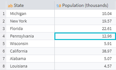
State population data
In the expression above, the second argument RowNumber is 3. In the image, the cell from in the fourth line is highlighted, because in Megaladata the row count starts from zero.
In the following screenshot from the Calculator node, newly calculated columns named after expressions Expr1, Expr2, and Expr3 are added to the columns from the input set:

Input columns and new expression-based columns
For the initial columns from the input set (Col1 and Col2), you can use the Data function to access the value of any cell.
When it comes to newly added columns (Expr1, Expr2, and Expr3), the Data function can only access the values of expressions that were calculated before the current one, or the values of any expression in rows with numbers less than the current row number.
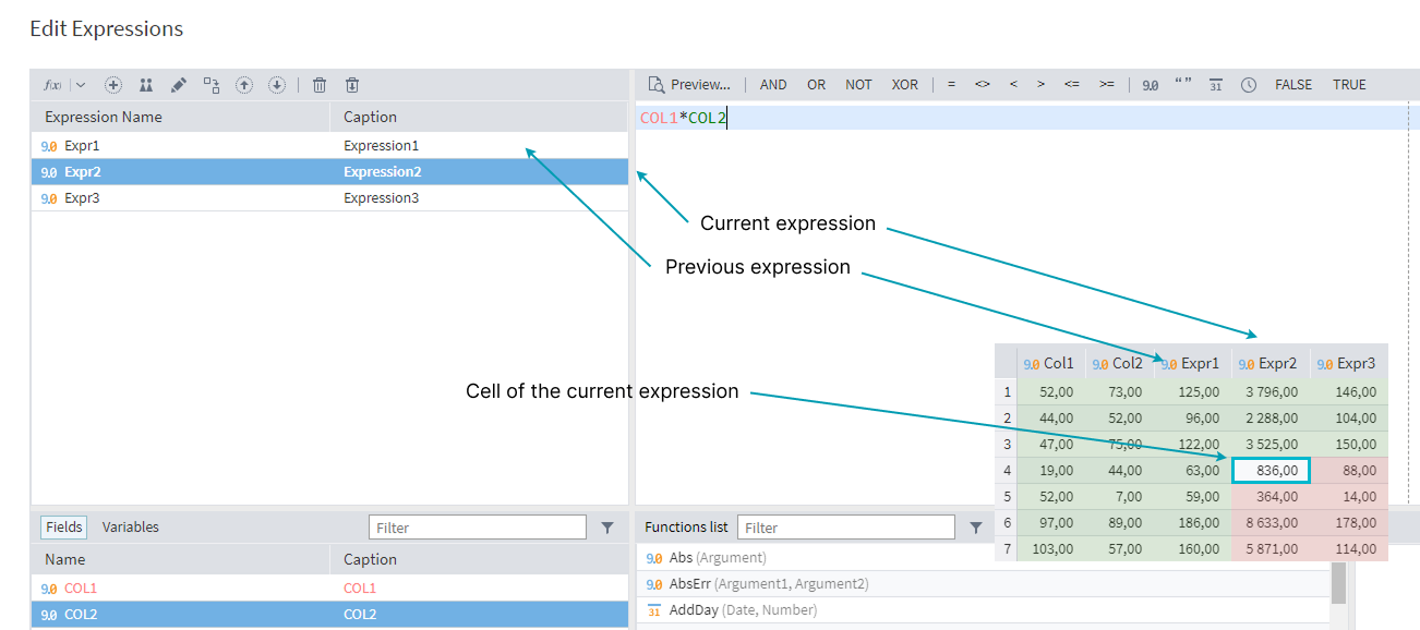
Editing expressions and previewing results
Here, the cells that the Data function can access when calculating the value of the current cell are highlighted in green; the cells that cannot be accessed are highlighted in red.
When working with the Data function, the following functions are almost always used to determine the row number:
- RowNum() returns the current row number
- RowCount() returns the number of rows.
Using these two functions involves some peculiarities that are important to know:
- To access the first row, use
0. - To access a row previous to your current row, enter
RowNum() - 1 - To access the row next to the current one, enter
RowNum() + 1. - To access the last row in your table, enter
RowCount() - 1(since the count starts from zero. E.g., if there are three rows in the table, the number of the last one will be 2).
When using this function recursively, it is important to select Cache in the Expression Parameters window:
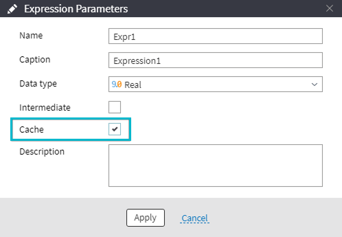
Expression parameters
This allows the function to remember previously calculated results, avoiding repeated calculations for identical queries.
Scenarios for using the Data function
As soon as it becomes clear that the values in one row are not enough, the need for the Data function arises. For better understanding, let's consider three use cases:
- Calculating the difference in price relative to the original price
- Change in sales compared to the previous day
- Filling in the gaps
Calculating the difference in price relative to the original
We have a table showing a product's price history. For each price listed, we need to calculate how much it has changed from the product's initial price.
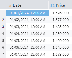
Daily prices
You need to find the difference between the current value and the value in the first row. If the Price column has the name Price, the expression in the Calculator should be the following:
Price - Data("Price", 0)
The formula calculates the difference between the current price value and the price value in the first row.
As a result, the Calculator adds a new column, which indicates how the price of the product has changed in relation to the original one.
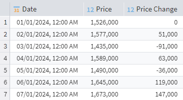
Calculated price change
Change in sales compared to the previous day
Another common task is to calculate the rate of change, where you want to know how much more or less you sold compared to the previous day. The input is a table containing information about the quantity of a product sold.
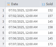
Daily units sold
To find out how sales have changed, you need to subtract the previous day's value from the current value. The difference will be positive if a larger quantity was sold on the current date, and negative otherwise. In our example, the Sold column has a name Sales, so the expression in the Calculator node is as follows:
IF(RowNum() = 0, 0, Sales - Data("Sales", RowNum() - 1))
This expression calculates the change in Sales relative to the previous row. If it's the first row (RowNum() = 0), it returns 0. Otherwise, it subtracts the previous row's value of Sales from the current row's Sales value. This calculation creates a new column showing the period-over-period change, assuming your data is sorted chronologically.
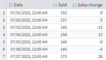
Calculated sales change
This is another example where one line of information is not enough. The task of finding the difference from the previous day essentially means you'd need to look one line up.
Using the Data Function to fill gaps
The Data function is also crucial for filling gaps in data arrays, a common challenge in areas like sales forecasting, where historical data is vital.
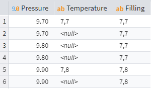
A typical example of this is filling empty cells with the last known value. Consider calculating the volume of gas in a pipeline, which requires both pressure and temperature measurements. One parameter, like pressure, might be measured every minute because it changes quickly, while the more inert temperature is only measured every five minutes. This results in a data table with intermittent gaps.
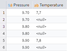
Data gaps
To calculate the volume, both values are needed. To fill in the gaps (i.e., Null values), you need to take the values from the previous rows. Given that the Temperature column's name is Temperature, the Calculator expression must be as follows:
IF(RowNum() <> 0 and IsNull(Temperature), Data("Filling", RowNum() - 1), Temperature)
This expression reads: if RowNum() <> 0, i.e. this is not the first row, and the Temperature value is empty (IsNull), return the value from the previous row of the new column Filling, otherwise, return the current value of column Temperature.
The result is a column labelled Filling, where all temperature reading cells are filled.
Filling in null values
While these are just three examples, the Data function is a key element in many other analytical tasks.
When not to use
As mentioned above, the Calculator usually works by rows and follows a simple logic: from each column, the value of a variable in the current row is considered. The Data function is essentially more resource-intensive, as it works with an entire array. Therefore, if there is no need to go beyond one row, it is better not to use it.
Also, we recommend opting out of using the Data function whenever there are dedicated handlers that can solve the problem easier.
For example, a common task is to combine all values from an input table column into a single, comma-separated string.
Let's consider a column labelled IP:
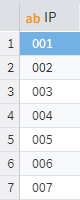
Sequential string values
To solve the task, you could use the Data function, writing the following expression in the Calculator node:
IF(RowNum() = 0, IP, Concat(Data("IP1", RowNum() - 1), ", " + IP))
This expression reads: if RowNum() = 0, i.e. this is the first row, return the value of the column with name IP. Otherwise, concatenate (combine into one row) the value from the previous row of the new IP1 column and the current value of the IP column, using a comma and a space as a separator.
As a result, new column IP1 will be added. Its last cell will have all values from the IP column, comma-separated.
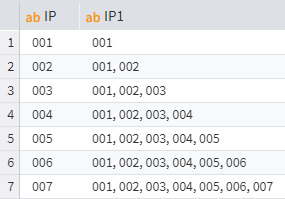
Cumulative concatenation of values
Now, you can extract that last value using the Grouping node:
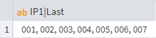
Grouping result
However, you can do the same transformation within the Grouping node immediately. Note that the data type at the node input must be string.
To get a comma-separated string, simply move the IP column to Parameters. (Double-click the column to open the Aggregation Options window and select List by marking the checkbox.)
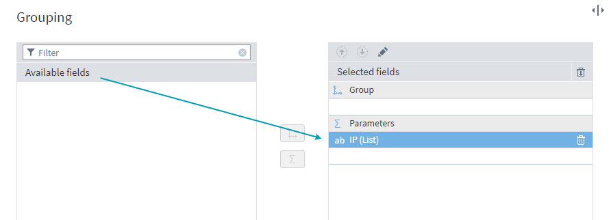
Creating a comma-separated string within the Grouping node
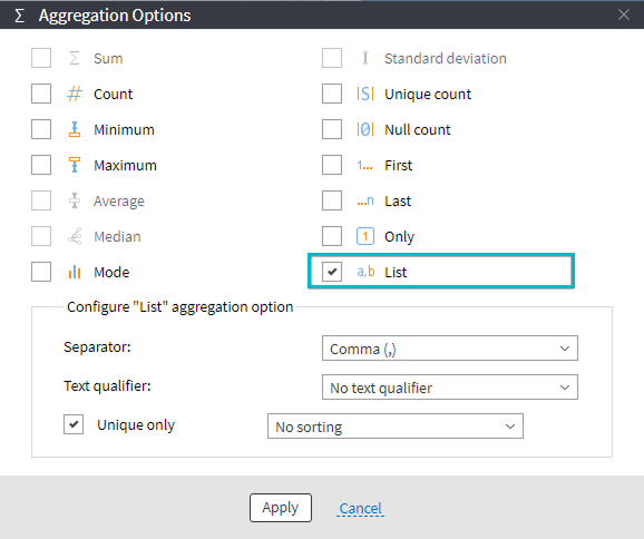
Selecting the List option
This way, you get the same result with just a couple of clicks:
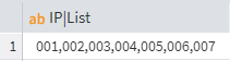
Result
Aggregation Options provide settings for handling most common tasks. You can choose different separators, sort data in ascending or descending order, or enclose values in single or double quotes.
Using quotes is particularly important for integrating with other applications. It helps you format data to meet the requirements of an external system. For example, you can convert column values into a set of key-value pairs for the JSON format.
However, for more specific or complex tasks, these standard options may not be enough—for instance, if you need a custom separator that isn't on the list or need to add a prefix to a value. In such cases, you can use the more versatile Data function instead.
For even greater flexibility, the Calculator node allows you to write custom JavaScript code. You can also call the Data function from within this code. Keep in mind that this approach uses more system resources, so it's best to stick with simpler solutions when possible.
Best practices for using the Data function
The Data function is a powerful tool, but using it correctly is key to building efficient workflows. Here are the most important things to consider:
- The
Datafunction can only be used inside a Calculator node. - Use this function only when you need to access data from multiple rows. If your data is in a single row, using it adds unnecessary overhead.
- Even when working with multiple rows, always check if a simpler, less resource-intensive solution exists before using the
Datafunction. - Pay close attention to syntax. Column names must be enclosed in quotation marks. Remember that rows are numbered starting from zero (e.g., the first row is '0', the second is '1', and so on).
- If using the function recursively (to call upon itself), you must enable the Cache option to ensure proper performance.
- The
Datafunction is almost always used in conjunction with theRowNum()andRowCount()functions. To correctly determine the number of the last row using theRowCount()function, remember that rows are numbered starting from zero. - The function can be used within JavaScript, which offers more flexibility but also increases resource consumption.
In summary, while the Data function is essential for certain analysis tasks, it's not always the best solution. Understanding its features and limitations will help you use it effectively and avoid common performance issues.
Read more:
See also

Megaladata at e-Logi Fest 2026

How Low-Code is evolving ETL
In 2026, you cannot scroll LinkedIn for five minutes without finding a post declaring "ETL is dead, ELT and AI have replaced it." It sounds compelling. It is also wrong.

Megaladata at Plug and Play Armenia Batch 3 Expo
On July 9, 2026, Megaladata took part in the Plug and Play Armenia Batch 3 Expo, the graduation event closing out the three-month International Pre-Acceleration Program in Armenia.
About Megaladata
Megaladata is a low code platform for advanced analytics
A solution for a wide range of business problems that require processing large volumes of data, implementing complex logic, and applying machine learning methods.
GET STARTED!
It's free